Implementing a model

In this section, an example of a full model implementation is given, using the 1977 paper “Reconstruction of the action potential of ventricular myocardial fibers” by Beeler and Reuter as our guide.

The complete article can be found here.

The model header

Every model definition starts with a header. This header consists of:

• The model name between double brackets, to indicate the start of the model definition section in the file.

• Any number of meta-properties

• The model’s initial state values

Here, we’ll name the model br1977 and add a description and a reference as meta data. The initial values will be added as we go along.

[[model]]
name: Beeler-Reuter 1977
desc: The 1997 Beeler Reuter model of the AP in ventricular myocytes
ref: """
Beeler, Reuter (1977) Reconstruction of the action potential of ventricular
myocardial fibres
"""

Time

Every myokit model needs a variable to represent time. You can call this “t” or “time” or “bob” as long as its explicitly defined. For example:

[environment]
t = 0
    in [ms]

Now to tell the simulation engine to use this as a time variable, we’re going to bind it to the external variable “time”:

[environment]
t = 0 bind time
    in [ms]

This asserts that the time variable should be bound to the external variable “time”. If no such variable is provided by the simulation engine, the default value 0 will be used.

The membrane potential

Like most models, the 1977 Beeler-Reuter model calculates the change in membrane potential as a function of the sum all trans-membrane currents. In myokit, this will look something like this:

[membrane]
C = 1 [uF/cm^2] : The membrane capacitance
dot(V) = -(1/C) * ( ??? )
    in [mV]
    desc: Membrane potential

Here, the equation for V is taken from equation (8) in the paper. The ??? part will be replaced by the names of the currents as we fill them in.

We’ve defined V as a state variable here, so we’ll need to add an initial value. The updated header becomes:

[[model]]
name: Beeler-Reuter 1977
desc: The 1997 Beeler Reuter model of the AP in ventricular myocytes
ref: """
Beeler, Reuter (1977) Reconstruction of the action potential of ventricular
myocardial fibres
"""
# Initial values:
membrane.V = -80

The given value for V is a reasonable guess. Once the model is implemented we can pace for a large number of beats to obtain a new set of initial values on a steady orbit.

Adding currents

The BR1977 model uses a single equation template for all currents. This means we could implement it quickly by defining a template equation and using it for every current.

However, if you look at the table given at the bottom of page 181, you’ll see quite a few zeros and ones, which greatly simplifies the corresponding equations.

In this example, we’ll write every current’s equation out in full. Each current will be placed in its own component and given a description and a unit. The current’s “gates” will be added as state variables and their transition rates will be added as nested variables.

The fast Sodium current: INa

First off, we’ll create a component called ina (in lower case to save some typing effort):

[ina]

The current itself is given in equation (5):

[ina]
INa = (gNaBar * m^3 * h * j + gNaC) * (membrane.V - ENa)
    in [uA/cm^2]
    desc: The excitatory inward sodium current

For this to work we’ll need to add some of the missing variables. Some of these are listed just below equation (5):

gNaBar = 4 [mS/cm^2]
gNaC = 0.003 [mS/cm^2]
ENa = 50 [mV]

Note that we’re using a fixed Nernst potential and a slight leakage current!

Now let’s add the m-gate. This is given in the paper as a differential equation, so we add another state:

dot(m) = alpha * (1 - m) - beta * m

alpha = (membrane.V + 47) / (1 - exp(-0.1 * (membrane.V + 47))) beta = 40 * exp(-0.056 * (membrane.V + 72)) desc: The activation parameter

To reduce the number of times we have to type membrane.V, we define a local alias with:

use membrane.V as V

Our code for m now becomes:

dot(m) =  alpha * (1 - m) - beta * m
    alpha = (V + 47) / (1 - exp(-0.1 * (V + 47)))
    beta  = 40 * exp(-0.056 * (V + 72))
    desc: The activation parameter

The other two gates can be added in a similar fashion, giving us the final result for the ina component:

[ina]
use membrane.V as V
gNaBar = 4 [mS/cm^2]
gNaC = 0.003 [mS/cm^2]
ENa = 50 [mV]
INa = (gNaBar * m^3 * h * j + gNaC) * (V - ENa)
    in [uA/cm^2]
    desc: The excitatory inward sodium current
dot(m) =  alpha * (1 - m) - beta * m
    alpha = (V + 47) / (1 - exp(-0.1 * (V + 47)))
    beta  = 40 * exp(-0.056 * (V + 72))
    desc: The activation parameter
dot(h) =  alpha * (1 - h) - beta * h
    alpha = 0.126 * exp(-0.25 * (V + 77))
    beta  = 1.7 / (1 + exp(-0.082 * (V + 22.5)))
    desc: An inactivation parameter
dot(j) =  alpha * (1 - j) - beta * j
    alpha = 0.055 * exp(-0.25 * (V + 78)) / (1 + exp(-0.2 * (V + 78)))
    beta  = 0.3 / (1 + exp(-0.1 * (V + 32)))
    desc: An nactivation parameter

The state variables m, h and j need initial values. None are provided in the paper so we make another educated guess:

[[model]]
name: Beeler-Reuter 1977
desc: The 1997 Beeler Reuter model of the AP in ventricular myocytes
ref: """
Beeler, Reuter (1976) Reconstruction of the action potential of ventricular
myocardial fibres
"""
# Initial values:
membrane.V = -80
ina.m      = 0.01
ina.h      = 0.99
ina.j      = 0.99

The calcium current

Next up, we add the calcium current following equation (6). Again, we define an alias for membrane.V and make a guess for the initial values. The intracellular calcium also varies depending on the current according to equation (9). To this end we add another state variable and set the initial value to 2e-7, within the range described on page 190:

[isi]
use membrane.V as V
gsBar = 0.09
Es = -82.3 - 13.0287 * log(Cai)
    in [mV]
Isi = gsBar * d * f * (V - Es)
    in [uA/cm^2]
    desc: """
    The slow inward current, primarily carried by calcium ions. Called
    either "iCa" or "is" in the paper.
    """
dot(d) =  alpha * (1 - d) - beta * d
    alpha = 0.095 * exp(-0.01 * (V + -5)) / (exp(-0.072 * (V + -5)) + 1)
    beta  = 0.07 * exp(-0.017 * (V + 44)) / (exp(0.05 * (V + 44)) + 1)
dot(f) = alpha * (1 - f) - beta * f
    alpha = 0.012 * exp(-0.008 * (V + 28)) / (exp(0.15 * (V + 28)) + 1)
    beta  = 0.0065 * exp(-0.02 * (V + 30)) / (exp(-0.2 * (V + 30)) + 1)
dot(Cai) = -1e-7 * Isi + 0.07 * (1e-7 - Cai)
    desc: The intracellular Calcium concentration
    in [mol/L]

The Potassium currents

BR1977 contains a time-independent Potassium current, given by equation (2):

[ik1]
use membrane.V as V
IK1 = 0.35 * (
        4 * (exp(0.04 * (V + 85)) - 1)
        / (exp(0.08 * (V + 53)) + exp(0.04 * (V + 53)))
        + 0.2 * (V + 23)
        / (1 - exp(-0.04 * (V + 23)))
    )
    in [uA/cm^2]
    desc: """A time-independent outward potassium current exhibiting
          inward-going rectification"""

A second Potassium current, ix1, does have some time dependence:

[ix1]
use membrane.V as V
Ix1 = x1 * 0.8 * (exp(0.04 * (V + 77)) - 1) / exp(0.04 * (V + 35))
    in [uA/cm^2]
    desc: """A voltage- and time-dependent outward current, primarily
          carried by potassium ions"""
dot(x1) = alpha * (1 - x1) - beta * x1
    alpha = 0.0005 * exp(0.083 * (V + 50)) / (exp(0.057 * (V + 50)) + 1)
    beta  = 0.0013 * exp(-0.06 * (V + 20)) / (exp(-0.04 * (V + 333)) + 1)

Updating the membrane potential

Now that we have all currents, we can update the equation for the membrane potential:

[membrane]
C = 1 [uF/cm^2] : The membrane capacitance
dot(V) = -(1/C) * (ik1.IK1 + ix1.Ix1 + ina.INa + isi.Isi)
    in [mV]
    desc: Membrane potential

Adding a stimulus

The one thing still missing is a stimulus current. We’ll add this by binding to the pacing mechanism, which is exposed in the standard simulations as “pace”. This variable will be set by the simulation engine using whatever protocol we pass it:

[stimulus]
amplitude = 25 [uA/cm^2]
IStim = pace * amplitude
pace = 0 bind pace

Now we need to set a protocol for our model. To this end, we add a protocol section at the bottom of the file:

[[protocol]]
# Level  Start    Length   Period   Multiplier
1.0      100      2        1000     0

This describes a simple block pulse. Initially, it’s value will be 0.0. But at t=100, this will change: our protocol defines a level of 1.0 at this point that lasts for 2 time units before going down again.

To create a period signal, a period of 1000 is set. Using the multiplier field we could limit the number of pulses, but in this case we’ll set it to 0 to specify an infinite pulse train.

Finalizing the definitions

Following equation (8) we add the new stimulus current to the membrane and provide the last few missing initial values:

[[model]]
name: Beeler-Reuter 1977
desc: The 1997 Beeler Reuter model of the AP in ventricular myocytes
ref: """
Beeler, Reuter (1976) Reconstruction of the action potential of ventricular
myocardial fibres
"""
# Initial values:
membrane.V = -80
ina.m      = 0.01
ina.h      = 0.99
ina.j      = 0.99
isi.d      = 0.01
isi.f      = 0.99
ix1.x1     = 0.0005
isi.Cai    = 2e-7

[environment]
t = 0 bind time
    in [ms]

[stimulus]
amplitude = 25 [uA/cm^2]
IStim = pace * amplitude
pace = 0 bind pace

[membrane]
C = 1 [uF/cm^2] : The membrane capacitance
dot(V) = -(1/C) * (ik1.IK1 + ix1.Ix1 + ina.INa + isi.Isi - stimulus.IStim)
    in [mV]
    desc: Membrane potential

[ina]
use membrane.V as V
gNaBar = 4 [mS/cm^2]
gNaC = 0.003 [mS/cm^2]
ENa = 50 [mV]
INa = (gNaBar * m^3 * h * j + gNaC) * (V - ENa)
    in [uA/cm^2]
    desc: The excitatory inward sodium current
dot(m) =  alpha * (1 - m) - beta * m
    alpha = (V + 47) / (1 - exp(-0.1 * (V + 47)))
    beta  = 40 * exp(-0.056 * (V + 72))
    desc: The activation parameter
dot(h) =  alpha * (1 - h) - beta * h
    alpha = 0.126 * exp(-0.25 * (V + 77))
    beta  = 1.7 / (1 + exp(-0.082 * (V + 22.5)))
    desc: An inactivation parameter
dot(j) =  alpha * (1 - j) - beta * j
    alpha = 0.055 * exp(-0.25 * (V + 78)) / (1 + exp(-0.2 * (V + 78)))
    beta  = 0.3 / (1 + exp(-0.1 * (V + 32)))
    desc: An inactivation parameter

[isi]
use membrane.V as V
gsBar = 0.09
Es = -82.3 - 13.0287 * log(Cai)
    in [mV]
Isi = gsBar * d * f * (V - Es)
    in [uA/cm^2]
    desc: """
    The slow inward current, primarily carried by calcium ions. Called
    either "iCa" or "is" in the paper.
    """
dot(d) =  alpha * (1 - d) - beta * d
    alpha = 0.095 * exp(-0.01 * (V + -5)) / (exp(-0.072 * (V + -5)) + 1)
    beta  = 0.07 * exp(-0.017 * (V + 44)) / (exp(0.05 * (V + 44)) + 1)
dot(f) = alpha * (1 - f) - beta * f
    alpha = 0.012 * exp(-0.008 * (V + 28)) / (exp(0.15 * (V + 28)) + 1)
    beta  = 0.0065 * exp(-0.02 * (V + 30)) / (exp(-0.2 * (V + 30)) + 1)
dot(Cai) = -1e-7 * Isi + 0.07 * (1e-7 - Cai)
    desc: The intracellular Calcium concentration
    in [mol/L]

[ik1]
use membrane.V as V
IK1 = 0.35 * (
        4 * (exp(0.04 * (V + 85)) - 1)
        / (exp(0.08 * (V + 53)) + exp(0.04 * (V + 53)))
        + 0.2 * (V + 23)
        / (1 - exp(-0.04 * (V + 23)))
    )
    in [uA/cm^2]
    desc: """A time-independent outward potassium current exhibiting
          inward-going rectification"""

[ix1]
use membrane.V as V
Ix1 = x1 * 0.8 * (exp(0.04 * (V + 77)) - 1) / exp(0.04 * (V + 35))
    in [uA/cm^2]
    desc: """A voltage- and time-dependent outward current, primarily
          carried by potassium ions"""
dot(x1) = alpha * (1 - x1) - beta * x1
    alpha = 0.0005 * exp(0.083 * (V + 50)) / (exp(0.057 * (V + 50)) + 1)
    beta  = 0.0013 * exp(-0.06 * (V + 20)) / (exp(-0.04 * (V + 333)) + 1)

[[protocol]]
# Level  Start    Length   Period   Multiplier
1.0      100      2        1000     0

Adding a plot script

All that’s left to do now is to add a simple plot script. This is written in plain python using the “magic” methods get_model() and get_protocol() to get the model and protocol from the gui. Then, a simulation is created and run:

[[script]]
import myokit
import matplotlib.pyplot as plt

# Get model & protocol from magic methods
m = get_model()
p = get_protocol()

# Create simulation
s = myokit.Simulation(m, p)

# Run simulation
d = s.run(1000)

# Display the result
t = d['environment.t']
v = d['membrane.V']

plt.figure()
plt.plot(t, v)
plt.show()

The resulting file can now be saved as a plain-text .mmt file and run using the GUI or myokit run. This example can be downloaded from here: br-1977.mmt

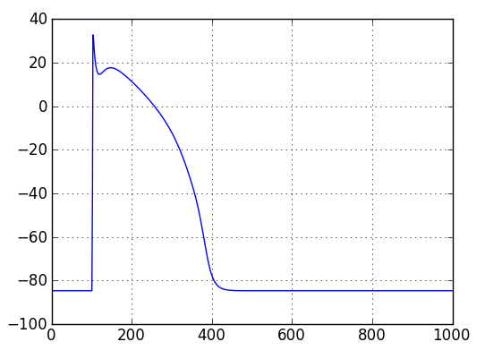
Result! A single action potential.