Running simulations

This section of the guide covers running simulations. To troubleshoot configuration or installation issues, check out the installation guide on the main page.

Getting started

There are two main ways of running simulations with myokit:

1. Using the GUI or myokit run to run the plot script embedded in an mmt file.

2. Using an independent python script that loads a model and protocol and creates a Simulation.

In the first scenario, you use the magic methods get_model() and get_protocol() to obtain the model and protocol from the other sections of the mmt file:

# Get model and protocol using magic methods
m = get_model()
p = get_protocol()

When running from an independent python script, you’ll need to get the model and protocol somwhere else, for example from a stored .mmt file:

import myokit

# Load a model, protocol and embedded script
m, p, x = myokit.load('example.mmt')

In the remainder of this document, we’ll assume you’re using myokit from an external script.

Creating a simulation

Myokit contains a number of simulation types, an overview of which can be found under API::Simulations. The most common types are:

• The single cell Simulation class, which uses the CVODES solver to perform high-speed single cell simulations.

• The multi-cell SimulationOpenCL class, which runs parallelised 1d or 2d simulations using a forward-Euler solver implemented in OpenCL.

All simulation types take a Model as first argument and a Protocol as optional second. Models and protocols passed into a simulation are always cloned. As a result, changes made to models or protocols after passing them to a simulation do not affect the simulation results.

Single cell example:

import myokit
m, p, x = myokit.load('example.mmt')
s = myokit.Simulation(m, p)

For multi-cellular simulations, the number of cells needs to be specified:

import myokit
m, p, x = myokit.load('example.mmt')
s = myokit.SimulationOpenCL(m, p, ncells=128)

For 2d simulations, use a tuple for the size:

import myokit
m, p, x = myokit.load('example.mmt')
s = myokit.SimulationOpenCL(m, p, ncells=(64, 64))

Additional arguments may need to be provided to multi-cellular simulations, for example the cell-to-cell conductance and the number of cells to receive an external pacing stimulus. For details, see the documentation of the appropriate simulation class.

Running and pre-pacing

To run a simulation, use the run(t) method. This advances the simulation t units in time and returns a myokit.DataLog object with the logged results. Internally, simulation objects maintain

• A time variable, representing the last time reached during simulation.

• A copy of the model state, representing the last state reached during a simulation.

• A copy of the model state, representing the model’s default state.

When a simulation is created, the time variable is set to zero and both the state and the default state are set to the values obtained from the simulation’s model. Every call to run(t) has the following effects:

• The time is moved t units ahead

• The simulation state is advanced t units in time.

• The default state is unaffected.

Example:

import myokit
m, p, x = myokit.load('example.mmt')
s = myokit.Simulation(m, p)

# The simulation time is now zero, the simulation state is the one returned
# by m.initial_values(as_floats=True)

log = s.run(1000)

# The simulation time is now 1000, the simulation state has been advanced
# 1000 units in time.

s.default_state() # Returns the original state
s.state()         # Returns the state at t=1000
s.time()          # Returns the new simulation time, t=1000

To undo the effects of one or more simulations, the model can be reset to its default state using the reset() method, which has the following effects:

• The time is reset to 0

• The simulation state is reset to the default state

• The default state is unaffected.

Example:

# Run the same simulation twice
import myokit
m, p, x = myokit.load('example.mmt')
s = myokit.Simulation(m, p)

d1 = s.run(1000)
s.reset()
d2 = s.run(1000)

# At this stage, d1 and d2 should contain the same values.

Frequently, a model needs to be “pre-paced” to a (semi-)stable orbit before running a simulation. This can be done using the method pre(t). Calls to pre() have the following effects:

• The time variable is unaffected

• The state has been advanced t units in time

• The default state has been advanced t units in time

This can be used to repeat the previous example, but now from a new starting point:

# Run the same simulation twice
import myokit
m, p, x = myokit.load('example.mmt')
s = myokit.Simulation(m, p)

# Pre-pace for a 100 beats
s.pre(100 * 1000)

# Run the same simulation twice
d1 = s.run(1000)
s.reset()
d2 = s.run(1000)

Manual changes to state, default state and time can be made using the methods set_state(), set_default_state() and set_time().

This approach is shared among all simulation types. For multi-cellular simulation the syntax for set_state() and set_default_state() is slightly more complex. This is explained in the corresponding documentation pages.

Logging

Each Simulation’s run() method returns a reference to a DataLog. This acts as a dictionary mapping variable qnames to data structures (typically lists or numpy arrays) containing the logged values:

import myokit
m, p, x = myokit.load('example.mmt')
s = myokit.Simulation(m, p)
d = s.run(1000)

import matplotlib.pyplot as plt
plt.figure()
plt.plot(d['engine.time'], d['membrane.V'])
plt.figure()

In this example, no special instructions were given to the Simulation about which variables to log. For large models or longer simulations it is often best to specify which variables to store. This can be done in a number of ways, the most common of which is to specify the variables explictly using their qnames:

d = s.run(1000, log=['engine.time', 'membrane.V'])

A shorthand is provided to log common variable types:

myokit.LOG_NONE

Don’t log anything

myokit.LOG_STATE

Log state variables

myokit.LOG_BOUND

Log bound variables (typically pace and time)

myokit.LOG_INTER

Log internal variables

myokit.LOG_ALL

Log everything

For example, to log all states and bound variables, use:

d = s.run(1000, log=myokit.LOG_STATE+myokit.LOG_BOUND)

Finally, an existing simulation log can be given as the log argument. In this case, new values will be appended to the existing log. This allows simulations to be run in parts:

import myokit
m, p, x = myokit.load('example.mmt')
s = myokit.Simulation(m, p)

# Run the first 500 ms, log states and bound variables
d = s.run(500, log=myokit.LOG_STATE+myokit.LOG_BOUND)

# Run the next 500ms, append to the log
d = s.run(500, log=d)

Post-processing

Once a simulation is done, the results can be saved to disk using the DataLog’s save_csv() method.

Alternatively, plots can be created from the logged data immediatly, without first storing the results. Myokit doesn’t depend on any particular plotting library, but for some quick tips on using the popular matplotlib library, see Visualization with Matplotlib.

For more examples of full simulations + post processing, check the Examples section of the myokit website.

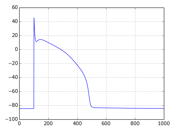
Example: Single cell

The following example uses the Luo-Rudy (I) model to create a plot of the action potential:

import matplotlib.pyplot as plt
import myokit

m, p, x = myokit.load('lr-1991.mmt')
s = myokit.Simulation(m, p)
d = s.run(1000)

plt.figure()
plt.plot(d['engine.time'], d['membrane.V'])
plt.show()

Result:

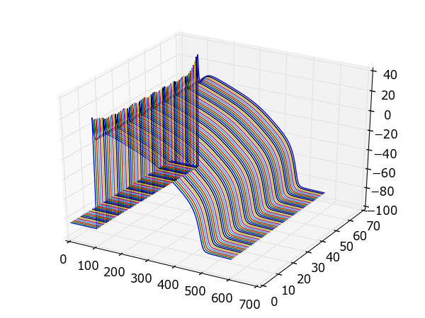
Example: A 1d strand of cells

The following example uses the same model in a strand simulation, and plots each trace side-by-side:

import matplotlib.pyplot as plt
import numpy as np
import myokit

m, p, x = myokit.load('lr-1991.mmt')
n = 64
s = myokit.SimulationOpenCL(m, p, ncells=n)
d = s.run(600)

from mpl_toolkits.mplot3d import axes3d
f = plt.figure()
x = f.gca(projection='3d')
z = np.ones(len(d['engine.time']))
for i in xrange(0, n):
    x.plot(d['engine.time'], z*i, d['membrane.V', i])
plt.tight_layout()
plt.show()

Result:

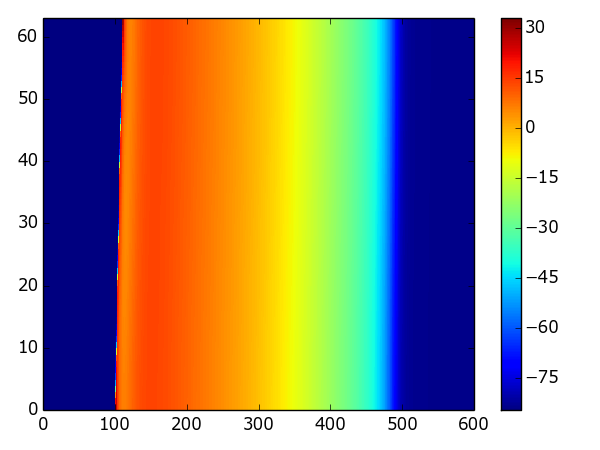
Example: A color-coded strand of cells

The following example uses the same model in a strand simulation, and plots the resulting voltages in a color-coded format:

import matplotlib.pyplot as plt
import numpy as np
import myokit

m, p, x = myokit.load('lr-1991.mmt')
n = 64
s = myokit.SimulationOpenCL(m, p, ncells=n)
d = s.run(600)
b = d.block1d()

x,y,z = b.grid('membrane.V')
f = plt.figure()
plt.pcolormesh(x,y,z)
plt.grid(False)
plt.xlim(0, np.max(d['engine.time']))
plt.ylim(0, n - 1)
plt.colorbar()
plt.tight_layout()
plt.show()

Result: